Home  /  Guide  /  Yagi antenna — construction

Guide · antennas · DIY

Building your own
2 m/70 cm Yagi antenna

Marian SQ4MN Technical consultationMarian SQ4MN · antenna designer

A few aluminium rods on a boom don’t add a single watt of power — they just squeeze it into a narrow beam. A station on the antenna’s axis will receive a signal 7 times stronger on 2 m and 11 times stronger on 70 cm than from a dipole, but much weaker to the sides and behind. Below are three complete designs: for 2 m, for 70 cm, and a handheld dual‑bander for satellites and the field. Each comes with millimetre‑accurate dimensions, a drawing, a shopping list, tuning instructions and a model file. I calculated all the antennas in the NEC‑2 simulator and checked how they tolerate build errors. These are computation‑based designs: the first built and measured example is still ahead of us.

2 m · 5 el. · 10.7 dBi 70 cm · 7 el. · 12.5 dBi 50 Ω without matching NEC‑2 model
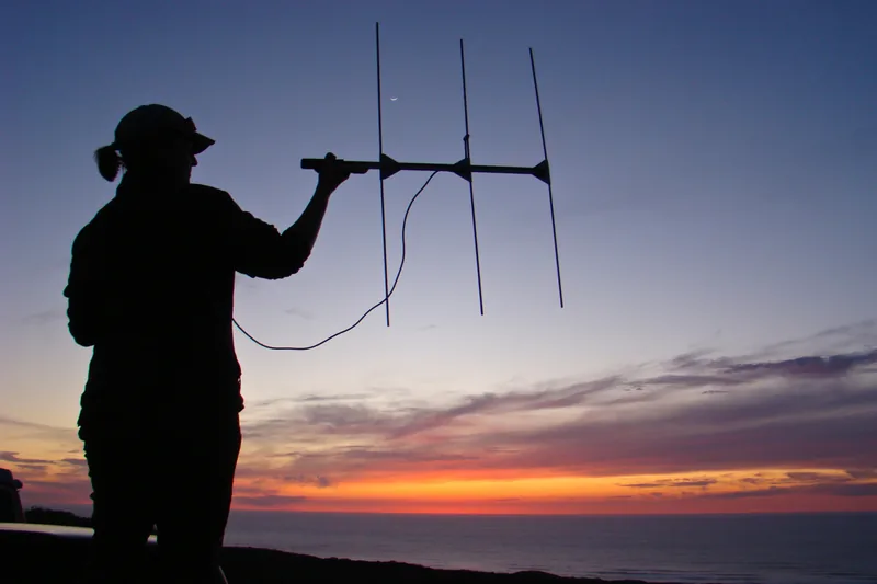
Silhouette of a person holding up a handheld three‑element Yagi antenna against an ocean sunset photo Lilian Carswell / USFWS · public domain · Commons
10.7dBi5‑element Yagi for 2 m
boom 1.7 m
12.5dBi7‑element Yagi for 70 cm
boom 1 m
≤ 1.24worst SWR in‑band, base antennas
(handheld ≤ 1.33)
±1mmcutting accuracy for 70 cm
for 2 m ±2 mm is sufficient
What’s the point

An antenna doesn’t amplify, it only focuses

An antenna has no power supply and doesn’t add a single watt. It radiates all the transmitter’s power just the same — only instead of sending it in all directions it steers most of it one way. To a station in the beam it looks as if an amplifier had turned 5 W into 35 W, but stations to the side and behind receive less than from a dipole. On receive it’s the same: the antenna doesn’t amplify the signal, it simply listens mainly in one direction, and less from the others, where noise and interference come from.

×7

Directional gain

8.6 dB over a dipole: in the beam axis the signal is as if the transmitter had seven times the power. The power doesn’t change, only its distribution, which is why gain is always “in some direction”.

F/B

Quiet at the back

A front–to–back of about 20 dB means signals and interference from behind the antenna are roughly a hundred times weaker.

∠

Direction finding

A narrow beam shows the direction. That’s how you go fox‑hunting, look for a source of interference and aim at a passing satellite.

PLN

Cheap and simple

No coils or capacitors: rods, boom, box and socket. Rods and boom are about 50 PLN for 70 cm and 70–135 PLN for 2 m.

The one on every roof

Everyone knows it from rooftops: a row of rods on a boom, the longest at the back, getting shorter towards the front. For half a century that’s what television antennas looked like, and that’s what most VHF/UHF directional antennas look like today, from amateur to early radars.

The idea is a hundred years old. From 1924 at the Imperial Tohoku University in Sendai, Hidetsugu Yagi and his assistant Shintaro Uda developed an antenna in which only one element is driven. The others, though not connected to the cable at all, operate from the neighbour’s field. Yagi patented it in 1926.

For a radio amateur it’s a dream homebrew project: there are no parts to buy from an electronics shop, apart from the socket, cable and ferrites. What you do have are dimensions — and that’s what everything depends on. I described the antenna’s history with a wartime anecdote on the SQ4MN dual‑bander.

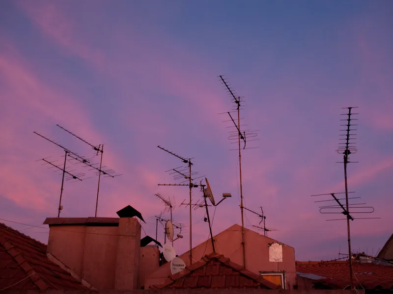
TV Yagi antennas on tenement rooftops against a pink sunset sky Yagi antennas on the rooftops of Lisbon’s Bairro Alto district · photo David Sim, CC BY 2.0, Commons
Physics without formulae

One driven, the rest work for free

The cable goes only to the driven element. The other elements take energy from its field and re‑radiate it with a phase shift. Lengths and spacings decide in which direction these waves will add up.

Currents in the elements of a Yagi antenna The cable is connected only to the driven element, but current flows in all elements. The current phase shifts from element to element, which is why the wave runs along the boom towards the directors. R DE D1 D2 D3 36%+113°84%±0°100%−122°96%−246°60%−372°currentphase beam →
RDED1D2D3
current36%84%100%96%60%
phase+113°±0°−122°−246°−372°
NEC‑2 simulation result for the 2 m (145 MHz) design. The thickness of the glow is the current magnitude, and the pulsing rhythm is its phase. The current in the reflector leads the driven element’s current by 113°, and the driven element’s wave reaches the reflector a further 59° late: together nearly 180°, so to the rear the waves cancel. In each subsequent director the current lags by another 122–126°, which is why the wave rides along the boom as if on rails and peels off at the front. An interesting detail from the bars below: the strongest current flows in the first director, not in the driven element to which the cable is connected. The driven element has only 84% of it.

Driven element only

dipole · 2.15 dBi
figure‑of‑eight, the same front and back

Plus reflector

2 elements · 6.5 dBi
back suppressed, front stronger

Plus three directors

5 elements · 10.7 dBi
narrow beam, back −22 dB

Plots to the same scale, common 0 dB = gain of the 5‑element antenna. Element positions as in the 2 m design.

R · reflector

The longest, at the back

About 0.49 wavelength. It is longer than resonant, so it is inductive: the current sets up with a phase such that it cancels the driven element’s wave to the rear and adds to it in phase at the front.

P · driven element

The only one with a cable

A centre‑fed dipole, about 0.48 λ. Its length chiefly sets the reactance at the feedpoint, i.e. the match to the cable.

D · directors

Shorter, at the front

0.41–0.45 λ. Each additional one narrows the beam, but the gain increases ever more slowly: on 70 cm five elements on a 0.45 m boom give 10.4 dBi in simulation, and seven on one twice as long give 12.5 dBi — only 2 dB more.

Glossary

Six terms, that describe an antenna

With each design below you’ll find the same parameters. Here’s how to read them:

dBi · dBd
Gain relative to an isotropic source (dBi) or a half‑wave dipole (dBd). The difference is always 2.15 dB: 10.7 dBi is 8.6 dBd. Diagram and catalogue pitfalls below the glossary.
F/B
Front–to–back ratio: how much weaker the antenna hears exactly from the rear. 20 dB is a hundred times less power.
−3 dB
Half‑power beamwidth: the width of the beam between the directions in which the power drops by half (−3 dB). The smaller the angle, the more precisely you need to aim.
SWR
Standing wave ratio. 1.5 is 4% reflected power, 2.0 is 11%. Below 1.5 the radio and the coax won’t complain.
E · H
Plot planes: E contains the elements, H is perpendicular to them. With the elements vertical (vertical polarisation) the E‑plane is vertical.
50 Ω
Impedance at the feedpoint. All three designs are close to 50 Ω, so you can connect the coax without a gamma or transformers.
Isotropic source, dipole and Yagi to the same scaleAn isotropic source radiates equally in all directions (a circle). A dipole radiates strongest broadside to itself (a figure‑of‑eight), 2.15 dB more than isotropic. A five‑element Yagi concentrates the same power into a narrow forward beam: 10.7 dBi, i.e. 8.6 dBd.isotropic source0 dBihalf‑wave dipole2.15 dBi = 0 dBdYagi 5 el. (2 m)10.7 dBi = 8.6 dBd
The distance of the envelope from the centre is the field strength in that direction, all three to the same scale; the dashed circle is the isotropic source. Each of these antennas radiates the same power. A dipole puts a bit less towards its ends, so broadside it has 2.15 dB more than the isotropic. A Yagi takes power from the sides and rear and sends it forwards. An isotropic source doesn’t exist; it’s a comparison standard: a point that radiates equally in all directions, like a light bulb hanging in a vacuum. The Yagi pattern is from the NEC‑2 model for 2 m, E‑plane.
pitfall 1

“dB” without a letter

The same antenna is 8.6 dBd and 10.7 dBi. When a catalogue lists just “dB”, it usually means dBi, i.e. a figure 2.15 higher. Only compare numbers in the same unit.

pitfall 2

Gain “with ground”

Ground reflection can add up to 6 dB in the best direction and is sometimes counted as antenna gain. That’s why the designs on this page are quoted in free space. Ask whether the gain is in free space.

pitfall 3

Gain you can’t get

A Yagi’s gain grows with boom length, not with the number of elements. Our 5‑element with a 1.7 m boom has 10.7 dBi, while seven elements on a 1‑metre boom on 70 cm give 12.5 dBi. A short boom with huge gain is a red flag.

Dimensions

Three designs, dimensions down to the millimetre

Pick an antenna. Each has a drawing, a dimensions table (base antennas in two rod diameters), simulation results and an NEC‑2 model file you can open in 4nec2 or any other NEC‑2‑compatible program.

Yagi 5 el. for 2 m

Base antenna: vertical for repeaters, horizontal for SSB. Boom 1.70 m, rods Ø 8 mm, and in the last column of the table a version with Ø 6 mm rods.

Dimensioned drawing of the 5 el. 2 m YagiFive elements on a 1.7 m boom; positions from the reflector 0, 336, 573, 1083, 1601 mm. centre of gravitymount only for horizontal polarisation R 1018 DE 992 D1 931 D2 924 D3 886 0 336 573 1083 1601 positions in mm from the reflector (always measure from the same point) radiation direction Yagi 5 el. · 144–146 MHz · rods Ø 8 mm

← drag the drawing sideways →

10.7 dBigain at 145 MHz (8.6 dBd)
22 dBfront–to–back at 145 MHz
50° · 63°−3 dB beamwidth: E · H
≤ 1.22SWR 144–146 MHz
1.70 mboom (5 cm past R and before D3)
≈ 1.3 kgweight with 20×20 boom
ElementPosition
from R [mm]
Length
Ø 8 [mm]
Length
Ø 6 [mm]
R · reflector010181023
P · driven element2 halves, gap approx. 10 mm336992996
D1 · director573931935
D2 · director1083924928
D3 · director1601886890

Lengths for a wood or plastic boom. With a metal boom add the correction to R and D from the “A metal boom shortens the elements” section. The driven element is measured end to end including the gap. This antenna is forgiving: an error of ±5 mm on all elements still gives SWR below 1.3.

SWR · NEC‑2

SWR of the 2 m antenna versus frequency SSB/CW repeaters 1.0 1.2 1.4 1.6 1.8 2.0 143 144 145 146 147 MHz

Solid line: rods Ø 8 mm, dashed: Ø 6 mm. Lighter band: 144–146 MHz.

Beam at 145 MHz

2 m antenna pattern at 145 MHz −3 −10 −20 −30 0° 30° 60° 90° 120° 150° 180° 210° 240° 270° 300° 330° front
E‑plane
in the plane of the elements · −3 dB: 50°
H‑plane
perpendicular · −3 dB: 63°
scale: 0 / −3 / −10 / −20 / −30 dB, 145 MHz
Download the NEC‑2 model

Yagi 7 el. for 70 cm

A narrow beam for distant repeaters and simplex contacts. Boom about 1 m, Ø 6 mm rods (one 1‑metre rod makes three elements); the last column of the table shows a Ø 4 mm version.

Dimensioned drawing of the 7‑element Yagi for 70 cmSeven elements on a boom about 1 m; positions from the reflector: 0, 81, 127, 274, 476, 704, 900 mm. centre of gravitymount only for horizontal polarisation R 342 DE 328 D1 303 D2 297 D3 289 D4 289 D5 283 0 81 127 274 476 704 900 positions in mm from the reflector (always measure from the same point) radiation direction Yagi 7 el. · 430–440 MHz · Ø 6 mm rods

← drag the drawing sideways →

12.5 dBigain at 435 MHz (10.4 dBd)
17 dBfront–to–back at 435 MHz
43° · 49°−3 dB beamwidth: E · H
≤ 1.24SWR 430–440 MHz
0.98 mboom (4 cm behind R and before D5)
≈ 0.58 kgweight with 20×20 boom
ElementPosition
from R [mm]
Length
Ø 6 [mm]
Length
Ø 4 [mm]
R · reflector0342344
P · driven element2 halves, gap approx. 10 mm81328330
D1 · director127303305
D2 · director274297299
D3 · director476289291
D4 · director704289291
D5 · director900283285

Lengths for a wooden or plastic boom; the correction for metal is in “A metal boom shortens the elements”. On 70 cm it’s better to be a few millimetres short than long: passive elements 7 mm shorter give SWR about 1.5, 7 mm longer give SWR 3.9 at 440 MHz.

SWR · NEC‑2

SWR of the 70 cm antenna versus frequency SSB repeaters 1.0 1.2 1.4 1.6 1.8 2.0 425 430 435 440 445 MHz

Solid line: Ø 6 mm rods, dashed: Ø 4 mm. Repeater inputs are 7.6 MHz lower, around 431–432 MHz.

Beam at 435 MHz

Radiation pattern of the 70 cm antenna at 435 MHz −3 −10 −20 −30 0° 30° 60° 90° 120° 150° 180° 210° 240° 270° 300° 330° front
E‑plane
in the plane of the elements · −3 dB: 43°
H‑plane
perpendicular · −3 dB: 49°
scale: 0 / −3 / −10 / −20 / −30 dB, 435 MHz
Download the NEC‑2 model

Handheld 2 m + 70 cm

Three elements on 2 m and six on 70 cm on a single wooden boom. For satellites, foxhunting and operating with a portable radio.

Dimensioned drawing of the handheld dual‑band antennaThree elements for 2 m and 6 elements for 70 cm on a common boom, in perpendicular planes. R2 1009 R7 346 P7 326 D7.1 305 D7.2 298 P2 969 D7.3 294 D2 878 D7.4 284 0 39 144 228 381 408 615 761 798 positions in mm from the reflector (always measure from the same point) radiation direction Handheld 2 m + 70 cm · wooden boom

← drag the drawing sideways →

7.8 dBigain on 2 m (145 MHz)
11.7 dBigain on 70 cm (435 MHz)
19 · 22 dBfront‑to‑back 2 m · 70 cm
≤ 1.33SWR 144–146 MHz
≤ 1.33SWR 430–440 MHz
0.86 m20×20 wooden boom
ElementPosition
from R2 [mm]
Length
[mm]
Rod
R2 · 2 m reflector01009Ø 6
R7 · 70 cm reflector39346Ø 4
P7 · 70 cm driven element2 halves, gap about 10 mm144326Ø 4
D7.1 · 70 cm director228305Ø 4
D7.2 · 70 cm director381298Ø 4
P2 · 2 m driven element2 halves, gap about 10 mm408969Ø 6
D7.3 · 70 cm director615294Ø 4
D2 · 2 m director761878Ø 6
D7.4 · 70 cm director798284Ø 4

The 2 m elements (Ø 6 mm) lie in one plane, and the 70 cm elements (Ø 4 mm, shown in green) in the perpendicular plane; in the drawing I’ve rotated them by 90° so you can see them. In reality, looking at the end of the boom, the elements of both bands form a cross (see the view in Satellites, foxes and summits). The boom is wood, so no correction. Each band has its own driven element and its own cable.

SWR · 2 m section

SWR of the 2 m section sat 1.0 1.2 1.4 1.6 1.8 2.0 143 144 145 146 147 MHz

SWR · 70 cm section

SWR of the 70 cm section satellites 1.0 1.2 1.4 1.6 1.8 2.0 425 430 435 440 445 MHz

Each band is calculated with the other band’s elements on the boom. In the model the bands don’t interact thanks to the perpendicular planes; in the real antenna the cables and imperfect assembly spoil this a bit.

Download the NEC‑2 model
Shopping and tools

Shopping list for one afternoon

You can buy everything at a DIY store and an electronics shop. There’s just one pitfall: the rod length.

Aluminium, not steel

Rods. The reflector for 2 m is over a metre long, and at Castorama the Ø 4, 6 and 8 mm rods are only 1 metre (9.98 PLN for Ø 6, 16.98 PLN for Ø 8). OBI has 2‑metre Ø 6 mm rods (GAH Alberts, 18.49 PLN), and wholesalers of aluminium and online shops sell Ø 6 and Ø 8 mm in 2 m lengths (about 13–14 PLN). For 70 cm, 1‑metre rods are enough: you get three elements out of one.

Boom. 20×20 mm square tube (for 70 cm 15×15 will do) in aluminium in 2 m lengths. Prices vary: 20×20 at OBI about 30 PLN, at Castorama 94 PLN for a thick‑walled 20×20×1.5 mm tube. Alternative without correction: an impregnated and varnished wooden batten or a plastic tube.

Fasteners. Stainless A2 or A4 screws, preferably with nylon spacers and washers. Stainless steel in aluminium is a galvanic couple: the aluminium around the screw can corrode, and water running off copper is particularly harmful to aluminium. Do not make elements from steel or bare copper.

Feed. Small IP65 sealed plastic box (the socket should end up right next to the driven element terminals), panel‑mount N socket (on 70 cm an N is more dependable than UHF/SO‑239), low‑loss cable to the radio (H‑155 for short runs, thicker for longer; RG‑58 only on a handheld) with a dense copper braid, including tinned copper, not copper‑clad aluminium (marked CCA), which solders poorly and quickly loses contact in the connector, 2–4 ferrite cores on the cable and neutral silicone, not acetoxy.

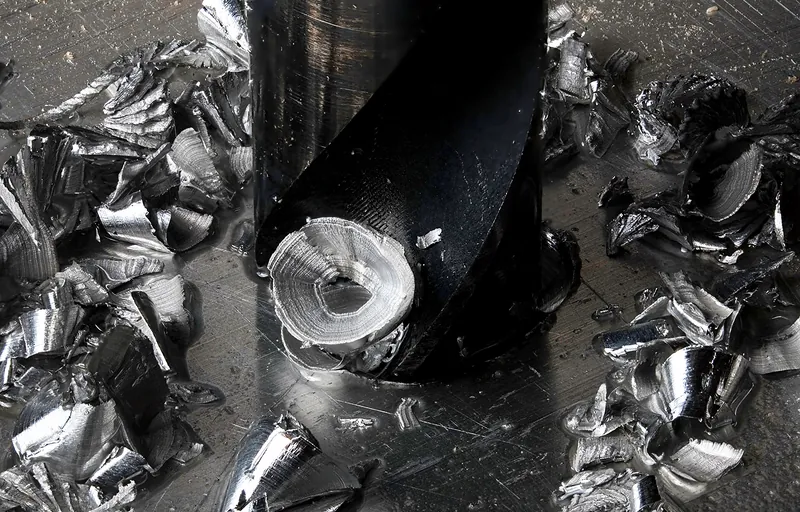
A high‑speed steel drill biting into aluminium, shiny swarf around it and a drop of lubricant HSS drill in aluminium, pillar drill, methylated spirits as lubricant · photo: JJ Harrison, CC BY-SA 3.0, Commons

← move the table sideways →

What2 m · 5 el.70 cm · 7 el.handheld 2 m + 70 cm
Aluminium rodsØ 8 mm, 3 × 2 mØ 6 mm, 3 × 1 mØ 6 mm 2 × 2 m + Ø 4 mm 2 × 1 m
Boom20×20 mm, 2 m15×15 or 20×20 mm, 1 m20×20 mm batten, 1 m (wood)
Mounts, bushings5 sets (or none if using wood)7 sets—
Box + socketsmall IP65 + Nsmall IP65 + N2 × small box + 2 × BNC or N
Ferrites2–3 × mix 433–4 × mix 612–3 × mix 43 (2 m) and 3–4 × mix 61 (70 cm)
Mast clamp2 U‑bolts2 U‑boltshand grip

Prices in the text are from September 2026, indicative. Tools: hacksaw, file, steel tape measure and calliper, drill (ideally a pillar drill), 3–8 mm bits (larger for the bushings), screwdrivers, soldering iron for the socket.

The most important correction

A metal boom shortens the elements

The dimensions in the tables are for antennas with no metal near the elements, i.e. on a boom of wood or plastic. A metal boom, even when the element doesn’t touch it, electrically “eats” part of its length and you need to give it back by adding a few millimetres.

Element passed through a boom of plastic or woodwood · PVC · GRPelement

Boom of wood or plastic

Dimensions from the table unchanged. The simplest route, especially on 70 cm.

correction: 0 mm
Element in an insulating mount above a metal boomPA6 GF30 mount, M3 screw3–4 mm above the boom

Mounts above the boom

WiMo/Konni‑type insulators in PA6 with glass fibre, element on an M3 screw, 3–4 mm above the boom. Measurements by DG7YBN; other mounts have a different correction.

+4 mm on 2 m · +7.5 mm on 70 cm
Element through a metal boom in insulating bushingsplastic bushings in the boom wallsno contact with metal

Through the boom, in bushings

Element insulated from the boom. According to DL6WU/G3SEK, half the full correction.

+3 mm on 2 m · +7 mm on 70 cm
Element through a metal boom, screwed, with electrical contactscrew or rivet, full contactscrew

Through the boom, with contact

The simplest to make, but the ARRL considers it the weakest unless the elements are welded: vibration enlarges the holes, and a loose element already has a different correction.

+6 mm on 2 m · +14 mm on 70 cm

Where do these millimetres come from

The correction was measured by DL6WU, and G3SEK expressed his chart as a formula, which today’s Yagi calculators use. What matters is the boom thickness relative to wavelength, so on 70 cm the same boom gives more than twice as much correction as on 2 m. Add the correction to the entire element length, half on each side.

Sources differ by 1–2 mm (square counted as a circle or as a circle 1.18 times thicker, wall thickness, distance from the boom end). On 2 m it’s irrelevant, as the design tolerates ±5 mm. On 70 cm the correction is larger than the antenna’s entire tolerance, so there I recommend a wood or plastic boom, or checking the antenna with an analyser after assembly.

The driven element is always insulated, as its halves go to the box. Authors don’t agree here, so the safest route is to do as DK7ZB does: leave 2 mm spare on each side and trim after measurement.

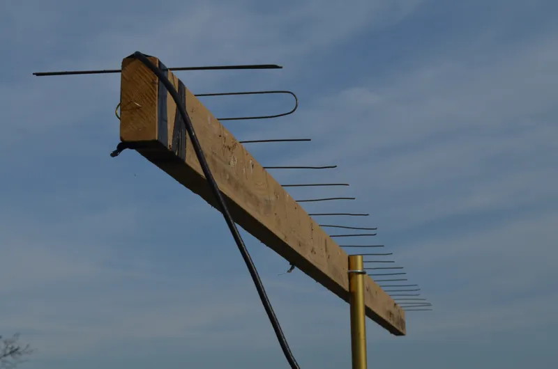
A home‑made wire Yagi on a wooden boom, a folded dipole at the end, sky in the background Makeshift UHF Yagi from clothes‑hanger wire on a wooden batten · photo: B137, CC BY-SA 4.0, Commons

← move the table sideways →

Mounting2 m, boom 20×2070 cm, boom 20×202 m, 15×1570 cm, 15×15
Wood, plastic0000
WiMo/Konni clamps, 3–4 mm above the boom+4+7.5+2.7+4.8
Through‑boom, insulated+3+7+1.8+4.4
Through the boom, with contact+6+14+3.5+8.8

Millimetres to be added to the total length of the parasitic element. Clamps: DG7YBN’s measurements for WiMo/Konni‑type insulators (PA6 GF30, M3 screw); for other clamps on 70 cm with a 20×20 boom he gives 3.4 to 5.6 mm, so in that case check the antenna with an analyser. Others: the DL6WU/G3SEK formula for a square treated as a circle of diameter 1.18 × the side length; VK5DJ’s calculator gives values differing by less than 1 mm, and DJ9BV gives, for insulated elements on a 20×20 boom, smaller values: 2 and 5 mm. No correction is applied to the driven element.

Driven element and cable

50 Ω straight to the cable plus a choke

I designed all three antennas so that the driven element is about 50 Ω. You don’t need a gamma, loop or quarter‑wave transformer. Just split the driven element in two and fit ferrites.

Why ferrites are mandatory here

In the designs on this page the split driven element goes straight to 50‑Ω cable. The dipole is balanced and the coax isn’t. Without a choke some current returns on the outside of the braid and the cable starts to radiate as an extra element: the beam skews, the backlobe grows, and the SWR changes when you move the cable or change its length.

Ferrite cores fitted as close to the driven element as possible choke this current. Current on the braid starts to flow at the feedpoint, so every centimetre of cable before the choke can radiate, and on 70 cm 17 cm is already a quarter‑wave. Fair‑Rite specifies mix 43 for attenuation from 20–250 MHz, and 61 above 200 MHz, so on 2 m use 43, on 70 cm 61. Jim Brown K9YC advises aiming for 500–1000 Ω impedance for current on the braid. A mix 43 Fair‑Rite 2643625202 core for cable up to 7.9 mm shows 361 Ω at 100 MHz and 415 Ω at 250 MHz per the catalogue, so on 2 m two are enough, three for margin.

Choke test: connect an analyser and grab the cable by hand a few tens of centimetres from the box. If the SWR twitches, current is flowing on the braid. Add another core.

Feeding the driven elementThe two halves of the driven element enter a sealed box. The N socket’s centre conductor connects to one half, the braid to the other. Ferrite cores sit on the cable as close to the driven element as possible, then the cable runs along the boom and forms a drip loop.halfof the driven elementhalfof the driven elementgap≈ 10 mmholedrainboominner → upperhalfbraid → lowerhalfN socketferritesas close as possibleof the driven elementdrip loop,cable to mast
Measure the driven element halves together with the gap: the length in the table is the end‑to‑end dimension. Connections inside the box: on 70 cm at most a few millimetres, on 2 m about 1 cm.

Short leads inside the box

The leads between the socket and the driven element terminals are not ‘a little wire’, they’re part of the antenna. Two wires 1 cm apart behave like a line of about 300 Ω and add inductance that shortening the driven element will no longer compensate. I ran the numbers in NEC‑2: on 70 cm as little as 2 cm of wire gives an SWR around 3, and by 8 cm the antenna stops working.

Limit: unshielded ends on 70 cm no more than a few millimetres, on 2 m about 1 cm. That’s why the box should be small and the socket right by the terminals.

Bigger box? Don’t run loose wires inside; bring the coax right to the terminals instead: the antenna cable through a gland, or a short length of coax (e.g. RG‑316) from the socket. A 50‑ohm section doesn’t spoil the match — only the unshielded end matters. You then fit the ferrites on that coax right by the terminals, because the current on the braid starts at the dipole, not at the socket.

Leads inside the boxSWR 2 mSWR 70 cm
0 (model)1.221.23
1 cm1.411.90
2 cm1.693.10
3 cm2.024.95
5 cm2.8810.5
8 cm4.6221.9

Worst in‑band SWR, NEC‑2 simulation of the designs on this page. The leads are modelled as a two‑wire line in air: wires Ø 1.5 mm with 10 mm spacing, i.e. about 310 Ω.

← move the table sideways →

Feed methodHow it worksNotes
Direct 50 ΩSpacings chosen so that the split driven element is about 50 ΩThe designs on this page. A ferrite choke is required.
Folded dipole + λ/2 balunA folded dipole has about four times the impedance of a plain driven element (for a 4:1 balun you design for about 200 Ω); a length of coax λ/2 × VF made into a loop gives a 4:1 transformationVoltage balun, not a choke. At 145 MHz about 682 mm, at 435 MHz about 227 mm with VF 0.66. A section cut per the catalogue VF usually resonates 5–10% low (DG7YBN), so check it with an analyser. This is how Marian SQ4MN feeds his antennas, described below. Make the loop from coax with a copper braid and solder carefully: sloppy joints spoil the match and symmetry, and then part of the power is lost in the loop and on the braid.
GammaDriven element intact, cable connected via an adjustable arm and a capacitorYou can tune it without cutting the rods, but the capacitor and slider must be adjusted and properly sealed.
DK7ZB28‑Ω driven element, two 75‑Ω cables in parallel as a λ/4 transformerPopular and well‑proven. Owen Duffy’s measurements show that it is mainly a transformer and the balun action is weak; DG7YBN advises adding ferrite.
?

Myth: the cable must be a multiple of a half‑wave. You often hear that the cable from the antenna to the radio should be a length equal to a multiple of λ/2 multiplied by the velocity factor. With a 50‑Ω matched antenna and 50‑Ω cable the length doesn’t matter: the cable doesn’t change SWR, and the losses depend only on its type and the number of metres. With a mismatched antenna the length changes the impedance seen by the radio, but the SWR is still the same; the cable’s attenuation only pulls it down at the radio end.

A λ/2 section has one useful property: at its far end you see the same impedance as at the antenna. So it’s handy when you want to measure the antenna’s own impedance from the shack with an analyser, in the λ/2 balun from the table above, and when combining antennas into arrays. If the SWR changes when you add or remove cable, the length isn’t to blame but current on the braid: you’re missing a choke.

Marian SQ4MNSQ4MN variantMarian SQ4MN · this is how he feeds his antennas

Folded dipole and λ/2 loop

Marian SQ4MN feeds his Yagis differently from the designs on this page. The driven element is a folded dipole designed for about 200 Ω, and the 50‑Ω cable is connected via a balun made from a half‑wave loop, i.e. a 4:1 transformer.

The midpoint of the continuous leg of the dipole is at zero potential, so it is connected to the boom. In the same place the braids of the loop and the feed cable are tied together. The loop forces equal and opposite voltages on the two halves of the dipole, and the braid is joined where the voltage is zero, so hardly any current flows on the outside of the cable. With this feed a choke is not necessary. You can add ferrite as cheap insurance if the cable runs close to the elements.

Here length really matters — but the length of the loop, not the cable to the radio: λ/2 × velocity factor, with VF 0.66 about 682 mm on 145 MHz and 227 mm on 435 MHz. Check a loop cut to the catalogue VF with an analyser, and solder on coax with a copper braid. You cannot transfer the dimensions from the tables above straight to this variant, because a folded dipole needs different spacings than a split 50‑Ω driven element.

Folded dipole fed by a half‑wave loopA folded dipole of about 200 Ω. The centre of the continuous leg is bonded to the boom. The two ends of a loop made from coax of length half a wavelength times the velocity factor are connected to the dipole’s terminals; the braids of the loop and the feed cable are joined together and connected to the dipole centre. A 50‑ohm cable goes to the radio. ← boom, dipole centre folded dipole ≈ 200 Ω braids joined and connected to the boom λ/2 loop × VF 682 mm · 2 m 227 mm · 70 cm 50 Ω cable to the radio 200 Ω → 50 Ω (4 : 1)
Feeding the folded dipole as per Marian SQ4MN: a half‑wave loop as a 4:1 balun, the braids joined to the dipole centre on the boom.
Step by step

From rods to an antenna on the mast

Order matters. Most antennas get ruined at step three, when marking out the boom.

1

Print the sheet and decide on the mounting

The “Print dimension sheet” button below the table prints just the drawing and the dimensions. Choose how you’ll mount the elements and immediately add the correction from the table above to each passive element.

R, D1, D2… + correction · driven element unchanged
2

Cut long, file to size

Cut 1–2 mm longer, then file to length and round the ends. Measure with a steel tape or vernier calliper, always the same one. On 70 cm the tolerance is ±1 mm, on 2 m ±2 mm. Cut the driven element halves 2 mm longer, to trim after measurement.

3

Mark out from a single point

Measure all positions from the centre of the reflector, with a single tape measure placed once, to an accuracy of ±3 mm on 2 m and ±2 mm on 70 cm. Do not measure each spacing from the previous hole: four spacings with 1 mm error each add up to 4 mm at D3, and on 70 cm six spacings make it 6 mm.

0 → 1601 mm (2 m design)
4

Drill perpendicular

All elements must be parallel and lie in one plane. Best is a pillar drill or a guide. Start with a centre drill or a small bit, then the final size, with a drop of methylated spirits or paraffin.

5

Centre every element

Mark the middle of the rod and set it on the boom’s centreline. The halves on both sides must be equal to the millimetre. An element offset sideways spoils the symmetry: the beam skews slightly, and at the driven element the current on the braid rises.

6

Driven element and box

The driven element halves enter the box with a gap of about 10 mm and are screwed to the terminals. The pin of the N socket to one half, the earth to the other; keep the leads to only a few millimetres long on 70 cm and about 1 cm on 2 m, hence the box should be small. At the lowest point of the box (once mounted) drill a 3 mm drain hole.

7

Cable and choke

Ferrite cores as close to the driven element as possible: with a small box right by the socket, and when the coax enters the box, on it, right at the terminals. Route the cable along the boom to the mast, perpendicular to the elements, and tie it with cable ties. Before the cable drops down the mast, make a drip loop.

8

Seal it

Wrap the N connector with self‑amalgamating tape, over it UV‑resistant insulating tape. Seal the box gaps with neutral‑cure silicone. Acetic‑cure silicone releases acid and corrodes contacts.

9

Measure, trim, mount

I describe SWR measurement below. After tuning, mount the antenna on the mast with the polarisation in mind: with vertical polarisation the mast must not pass between the elements.

Marking out the boom: from a single point, not from the previous holeOn the left all dimensions measured from the reflector. On the right the spans measured from the previous hole, each with a 1 mm error, so the error grows to 4 mm on the last director.RDED1D2D3CORRECTfrom the reflector33657310831601WRONGfrom the previous one336+1237+2510+3518+41 mm error on each span → +4 mm at D3
Step 3 in practice. Always hook the tape in the same place, on the reflector axis. Measuring each spacing from the previous hole accumulates errors, and when correcting the boom it’s easy to make a mistake.
!

Safety at the mast. Erect the mast so that if it falls it can’t reach a power line. Earth the metal mast and the cable braid at the building entry. On the roof work with fall protection and never alone. I’ve described getting permission for an antenna on a housing association building in my guide about an antenna on the roof.

Measurement

NanoVNA will tell the truth

An antenna designed in a simulator and carefully built usually hits the mark straight away. Measurement is still mandatory: it will show a mistake in the correction, a bad contact and water in the connector.

How to measure so the result means something

Antenna skywards. Set the boom vertical, directors pointing up, at a height of at least two metres and away from metal. VK2KU measured all antennas like this, and DG7YBN advises there should be nothing in the beam within the nearest 20 metres. Measuring in a room or on a balcony by a wall shifts the resonance.

Cable in a loop. The cable should hang in a wide curve, not run along the antenna. Calibrate the analyser at the end of the cable, or remember that each decibel of cable loss inflates the measured return loss (RL) by two decibels (Owen Duffy).

What to use. NanoVNA‑H measures from 50 kHz to 900 MHz. Above 300 MHz it works on harmonics with lower dynamic range, but that’s perfectly sufficient for SWR on 70 cm. Newer NanoVNA‑H4 units reach 1.5 GHz. An SWR meter for 144/430 MHz and a radio are also enough, as long as you use several frequencies.

What to expect: a curve similar to the one in the design plot. If it’s the same shape, just shifted, it means the elements came out too long or too short. The table below suggests what to do.

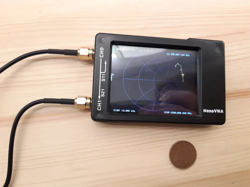
A NanoVNA analyser on a wooden surface with a Smith chart on the screen and two SMA leads NanoVNA with Smith chart · photo: Elgull, CC BY‑SA 4.0, Commons
What you seeWhat it means and what to do
On 2 m SWR above 1.5 anywhere in the bandIt’s not the driven element length: in simulation even ±10 mm gives at most 1.33. Look for a fault in the connections, in the box, in the choke or in the element positions.
On 70 cm SWR rises towards 430 MHzDriven element too long. Shorten both halves by 1 mm and measure again. A shorter driven element improves the bottom of the band at the expense of the top.
On 70 cm SWR rises towards 440 MHzDriven element too short or, more often, passive elements too long, e.g. from applying the boom correction twice. Passive elements longer by 7 mm give an SWR of about 3.9 at 440 MHz.
On 70 cm the whole curve is shifted by a few MHzAll elements too long (curve down) or too short (up). Each millimetre is about 1.2 MHz of shift.
SWR high everywhere, above 3Short or open in the box, leads from the socket to the driven element too long (on 70 cm even 2 cm gives an SWR of about 3), water in the connector, damaged cable or one half of the driven element shorted to the metal boom.
SWR changes when you move the cableCurrent on the braid. Add ferrite cores as close to the driven element as possible.
Good SWR, but poor gain and a large rear lobeSWR doesn’t measure directivity. Check the order and positions of the elements, and whether the directors are touching metal where they shouldn’t.
Installation

Vertical for repeaters, horizontal for SSB

The same antenna rotated by 90° changes polarisation. Choosing the wrong one can cost you as much as the whole design has gained.

Yagi with elements vertical: vertical polarisationE‑fieldvertical

Elements vertical

FM, repeaters, contacts with handhelds and mobile radios. IARU Region 1 Recommendation FM.24 is explicit: repeater antennas use vertical polarisation.

FM · repeaters · APRS
Yagi with elements horizontal: horizontal polarisationE‑field horizontal

Elements horizontal

SSB, CW, digital modes and contests. There’s no formal recommendation, but the IARU R1 VHF Handbook says we operate horizontally everywhere except on FM channels.

SSB · CW · FT8 · tropo

Mast and a vertical antenna

Between stations with different polarisations you lose 20 dB or more according to the ARRL. That’s a hundred times less power – more than the whole antenna gives you.

With vertical polarisation there’s a second trap: a metal mast running through the middle of the antenna is parallel to the elements and becomes one of them. I ran the numbers for the 2 m design with a 40 mm diameter metal mast: without the mast 10.7 dBi and front–to–back 22 dB; with the mast through the centre, depending on its length, from 10.4 down to just 7.8 dBi, and front–to–back drops even to 8 dB. With the mast 35 cm behind the reflector: 10.7 dBi and 23 dB, i.e. no change.

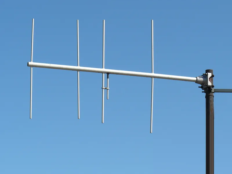
Solutions: mount behind the reflector (boom extended to the rear; on 2 m the boom comes out about 2.05 m or use a short extension), a side standoff, or a section of non‑metallic mast within the antenna. With horizontal polarisation the mast is perpendicular to the elements and causes little trouble. This is how the Radmor antenna from Gdynia in the photo is mounted: the boom is extended behind the reflector and its end bolted to the mast.

A four‑element Yagi with vertical elements against a blue sky, boom end‑mounted to the mast VHF directional antenna made by Radmor in Gdynia, elements vertical · photo: Zalasem1, CC BY-SA 4.0 (crop, overlay with nameplate removed), Commons
Metal mast through the middle of the antenna, parallel to the vertical elementsmetal mast7.8–10.4 dBimast through the centre · gain 7.8–10.4 dBi, F/B as low as 8 dB
Mast behind the reflector, boom extended to the rearmast behind the reflector10.7 dBimast behind the reflector · gain 10.7 dBi, F/B 23 dB
Surroundings

An antenna likes free space

In NEC‑2 the model hangs in a void. A real antenna has a wall, a gutter, a balcony railing and another mast nearby, and every bit of metal close to the elements starts acting like one more element.

“Most important: antennas like free space. When I kept the antenna clear of its surroundings, it really came to life.”Marian SQ4MN

I checked in NEC‑2 how far “far” is. I added metal parallel to the elements to the models on this page, because that’s what interferes most: a single 20 mm diameter tube about 3 λ long (gutter, another antenna’s mast, post) or a 2 × 2 λ metal wall made of rods spaced every 1/10 of a wavelength (sheet metal, mesh, railing, rebar). The result depends on which side the obstacle is on.

Front, i.e. the main lobe. Close in, SWR rises: a tube half a metre in front of the last director of the 2 m antenna gives SWR 1.9, and 20 cm in front of the 70 cm antenna it’s 2.0. On 2 m the SWR returns to normal from about ½ λ; on 70 cm only about 2 λ further away. Beyond that, metal in the beam still steals gain and worsens the back: a tube 20 m in front of the 2 m antenna is still −0.3 dB and F/B 19 instead of 22 dB. There should be nothing in the beam as far as you can manage.

Side, i.e. a wall along the antenna. This is where you lose the most, and an analyser won’t show it because SWR hardly changes. At a distance of ¼ λ the antenna loses over 4 dB, i.e. half of what it gives over a dipole. At ½ λ still 1–2 dB. From about 1 λ the on‑axis gain only wiggles by ±1 dB, because the reflection from the wall sometimes adds, sometimes subtracts. With horizontal polarisation a sheet‑metal roof under the antenna is also such a “side”.

Rear, i.e. behind the reflector. The reflector shields the antenna. A wall even ¼ λ behind it doesn’t change SWR, and the gain moves by at most ±1 dB. If you have to bring the antenna close to a building, do it at the back.

On a balcony point the antenna away from the wall, outwards, not along the facade. A railing with metal bars parallel to the elements acts like the wall in the table. Metal in the model is the worst case: brickwork and wood reflect less, but some energy is lost in them.


Free‑space clearances around a Yagi, top viewIn front and to the sides the antenna needs at least one wavelength free of metal; at the back a quarter‑wave is enough. In the beam in front of the antenna, metal still causes trouble further out.metal in the beam gets in the wayeven 10 λ further onfront ≥ 1 λside ≥ 1 λrear ≥ ¼ λ1 λ = 2 m on 2 m · 0.7 m on 70 cm¼ λ = 0.5 m · 0.17 mtop view, 2 m design scale

← move the table sideways →

Distance (2 m / 70 cm)2 m · 5 el.70 cm · 7 el.
Front: tube in the beam, distance from the last director
≈ ¼ λ (0.5 / 0.2 m)−0.8 dB · SWR 1.88−1.0 dB · SWR 2.01
≈ ½ λ (1 / 0.35 m)−1.1 dB · SWR 1.24−1.5 dB · SWR 1.60
1 λ (2 / 0.7 m)−0.8 dB · SWR 1.22−1.2 dB · SWR 1.40
10 λ (21 / 6.9 m)−0.3 dB · SWR 1.22−0.4 dB · SWR 1.24
Side: metal wall along the antenna, distance from the boom
¼ λ (0.5 / 0.17 m)−4.3 dB · SWR 1.33−4.8 dB · SWR 1.39
½ λ (1 / 0.35 m)−1.1 dB · SWR 1.21−1.8 dB · SWR 1.29
1 λ (2 / 0.7 m)+1.5 dB · SWR 1.21+0.9 dB · SWR 1.23
2 λ (4 / 1.4 m)−0.1 dB · SWR 1.20+0.1 dB · SWR 1.24
Rear: metal wall behind the reflector
¼ λ (0.5 / 0.17 m)−0.3 dB · SWR 1.23+0.3 dB · SWR 1.23
½ λ (1 / 0.35 m)+0.5 dB · SWR 1.21−0.3 dB · SWR 1.24
1 λ (2 / 0.7 m)+0.3 dB · SWR 1.22−0.7 dB · SWR 1.23
2 λ (4 / 1.4 m)0.0 dB · SWR 1.22−0.9 dB · SWR 1.23

Change in on‑axis gain relative to free space (10.7 and 12.5 dBi) and worst‑case SWR in the band, NEC‑2. With a wall to the side at 1 λ the on‑axis gain increases, but the beam splits into lobes, so this isn’t free gain. Bottom line: at least 1 λ of metal‑free space in front and to the sides (2 m on 2 m, 0.7 m on 70 cm), ¼ λ behind is enough.

Handheld version

Satellites, foxes and summits

The handheld dual‑band from project three is an antenna for operating on the move: you can track a satellite across the sky with it, hunt down a transmitter, or take it to a summit for SOTA.

Two bands on one boom

The 2 m elements lie in one plane and the 70 cm in a plane at right angles, all centred on the boom. The field of one band then has no component along the rods of the other, so it doesn’t induce current in them: in the NEC‑2 model the presence of the other antenna doesn’t change gain or SWR. In a real antenna that symmetry is upset by the cables and imperfect assembly, so run the cables along the boom and measure each band separately. You change polarisation with a twist of the wrist, which is an advantage with satellites because their signal changes polarisation anyway during the pass.

Two cables or a duplexer. The IC‑9700 and other radios with separate sockets for 2 m and 70 cm are connected with two cables. For a handheld radio with a single socket you need a duplexer, e.g. Diamond MX‑72N (paths 1.6–30/49–150 and 400–460 MHz, isolation at least 60 dB, losses up to 0.15/0.25 dB, up to 150/100 W) or Comet CF‑4160 (1.3–170 and 350–540 MHz). The manufacturer intends the MX‑72N for indoor and in‑car use.

Through the ISS repeater and the SO‑50 satellite you transmit on 2 m and receive on 70 cm. The satellite passes calculator shows when they pass over Poland, and I’ve described how to work them in the guide on satellite communications.

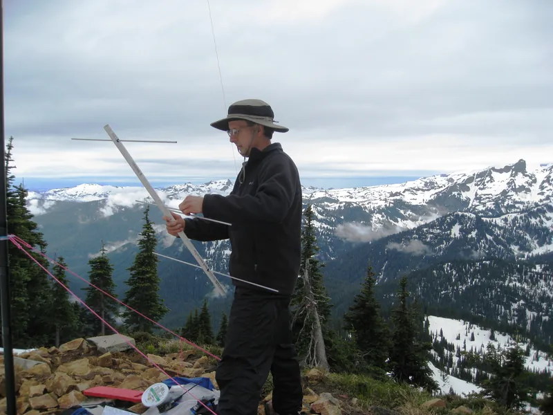
A radio amateur in a hat assembling a 2 m Yagi on a rocky ridge, snow‑capped mountains in the background Assembling a 2‑metre Yagi near Naches Peak, 1,919 m a.s.l. · photo: brewbooks, CC BY‑SA 2.0, Commons

One driven element or two?

You can build dual‑band Yagis in two ways. One driven element for both bands, e.g. a folded dipole or a trapped driven element, gives you a single feed but is harder to match on both bands at once. That’s how Marian SQ4MN built his dual‑band antenna with a copper dipole.

Two separate driven elements are used in popular handheld satellite antennas, e.g. Arrow II 146/437‑10: 3 elements on 2 m and 7 on 70 cm on one boom, each band with its own driven element and connector, with an optional diplexer in the handle. Here the bands lie in perpendicular planes, so from the front of the boom you see a cross.

The dimensions of the third design don’t come from any existing antenna. It’s my own optimisation in NEC‑2, not yet built; you can check the model in the downloadable file.

View from the front of the boom: 2 m elements horizontal, 70 cm elements vertical, together forming a cross 2 m elements 70 cm elements view from the front of the boom boom
Before you start

Ten mistakes that ruin a Yagi

All are cheap to avoid and expensive to find once the antenna is up the mast.

01

Adding up the spacings

Measuring from the previous hole accumulates errors. Always from the reflector.

02

Boom correction twice or not at all

On 70 cm with a 20×20 boom that’s 7–14 mm, more than the antenna’s tolerance. Note on the sheet, whether the dimension already includes the correction.

03

No choke

The cable radiates, SWR depends on its length, the beam runs off to one side. Ferrites as close to the driven element as possible.

04

Mast between elements

With vertical polarisation a metal mast becomes an extra element. Mount behind the reflector.

05

Measuring at ground level

An antenna on the lawn or leaning against a wall shows a false resonance. Measure with it pointing at the sky.

06

Water in the connector

An unsealed connector after winter can have green corrosion and an SWR of 3. Self‑amalgamating tape and a drain hole.

07

Steel and copper on aluminium

A galvanic couple eats the aluminium around the bolts. Nylon sleeves and washers, no steel rods.

08

Long leads in the box

8 cm of leads from the connector to the driven element means an SWR of about 20 on 70 cm. Coax right up to the terminals.

09

Test cable too long

Twenty metres of RG‑58 on 70 cm is nearly 7 dB of loss and an SWR that always looks great. Measure at the antenna.

10

Antenna in a tight corner

A metal wall ¼ wavelength to the side costs you over 4 dB, and SWR won’t show it. Leave 1 λ clear in front and to the sides, and face the back towards the wall.

Before you raise the mast

Checklist

Your ticks are saved in this browser, so you can come back to the list during the build.

Done: 0 / 9
A hundred years of the antenna

From Sendai to every rooftop

1924

Laboratory in Sendai

Hidetsugu Yagi and Shintaro Uda begin work on a directional antenna with parasitic elements. That’s what the IEEE Milestone plaque says.

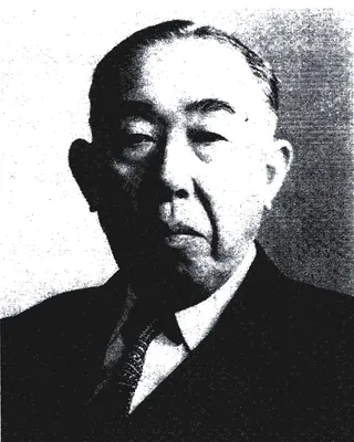
Portrait of Hidetsugu Yagi, 1953 Portrait of Shintaro Uda H. Yagi and S. Uda
photo: public domain
1926

Patents and papers

Yagi receives Japanese patent no. 69115 and files in the USA (patent 1,745,342, granted in 1930). Uda publishes, in Japanese, a series of papers “On the Wireless Beam of Short Electric Waves” (1926–1929).

1928

The world finds out

In the June issue of “Proceedings of the IRE” Yagi publishes “Beam Transmission of Ultra Short Waves”. Hence the colloquial name: Yagi, though strictly it’s Yagi‑Uda.

1995

Milestone

On 17 June the IEEE unveils the “Directive Short Wave Antenna, 1924” plaque at Tohoku University in Sendai. Today the same principle is used by millions of antennas, from television to radio astronomy.

From our band

Marian SQ4MN’s Yagi

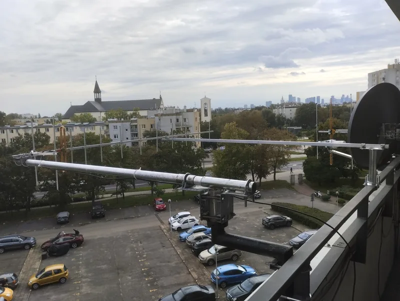
Marian SQ4MN builds antennas himself and puts them up on his balcony in Warsaw. His 70 cm has an extra support under the boom, and from the elements left over from two antennas he also put together a dual‑band antenna with a copper folded dipole.

It’s good proof that a Yagi doesn’t need a workshop: rods, a boom and patience with measuring are enough. I’ve described both builds on separate pages: 70 cm Yagi with a second support and antenna for 2 m and 70 cm.

Marian SQ4MN’s 70 cm Yagi on a balcony, boom with an additional support Marian SQ4MN’s 70 cm Yagi · photo: Marian SQ4MN

Sources and method

  1. Dimensions: my own optimisation in NEC‑2 (nec2c), free‑space model, aluminium σ = 2.5·10⁷ S/m, extended thin‑wire kernel, 41 segments per half‑wavelength, convergence checked up to 81 segments. Tolerances: 400 random antennas with length and position errors.
  2. Boom correction: G3SEK, DL6WU Yagi — DIY (G3SEK formula based on DL6WU measurements); DG7YBN, Boom Correction; VK5DJ, YagiCalculator (GPL source code); DK7ZB, construction details.
  3. Ferrites: Fair‑Rite, material datasheets 43 and 61, core 2643625202; J. Brown K9YC, “A Ham’s Guide to RFI, Ferrites, Baluns, and Audio Interfacing”. Baluns: DG7YBN; DK7ZB match and measurements by Owen Duffy.
  4. Polarisation: IARU Region 1, VHF Handbook v10.03 (February 2026, recommendation FM.24); ARRL Antenna Book, ch. 18.
  5. Measurements: VK2KU, “Effects of Boom and Element Diameters on Yagi Element Lengths at 144, 432 and 1296 MHz”, QEX, January/February 2000; DG7YBN, antenna VSWR measurements; NanoVNA‑H documentation (hugen79).
  6. History: IEEE/ETHW, Directive Short Wave Antenna, 1924; H. Yagi, Proc. IRE 16(6), 1928; US patent 1,745,342.
  7. Antenna surroundings: my own NEC‑2 calculations of the models on this page with a Ø 20 mm tube (length approx. 3 λ) and a 2 × 2 λ wall made of Ø 4 mm rods spaced at λ/10, parallel to the elements. Dual‑band: Arrow II 146/437, manufacturer’s datasheet.
  8. Technical consultation: Marian SQ4MN, notes from 22.09.2026 (an antenna is not an amplifier, dBi and dBd, cable quality, free space around the antenna, source of the dual‑band design, feeding a folded dipole via a λ/2 loop without a choke).
  9. Duplexers: product sheets for Diamond MX72N and Comet CF‑4160. Material prices: Castorama, OBI, metalnow.pl, as of 21.09.2026.

The NEC model doesn’t know your boom, mounts, junction box or surroundings, so it’s the measurement of the finished antenna that always has the final say.

Next step

Calculate how far it will reach

Enter the new antenna’s gain, power, cable and mast height, and the calculator will show range and EIRP. You can check cable losses in the cable calculator.